|
|
|
Stefano Chimichi-NMR Guide |
Department
of Chemistry
|
|
Resources
|
Welcome
to the User Resource Guide for the NMR (Small Molecules) at
the Chemistry Dept of the
University of Firenze. This guide will help you navigate the facility
and use the instruments for standard and advanced NMR techniques. Please choose the desired experiment or technique from the list
below or scroll down the page to browse listings.
|
|
|
|
|
|
|
|
|
|
|
|
|
How
do I....
|
|
|
|
|
|
|
|
|
|
|
|
|
|
|
|
|
|
|
|
|
|
|
|
|
| |
|
|
| |
Run a 90-Degree Pulse
Width Calibration |
|
Note: Bold text represent boxes
you should click. italic
text represent text you
should type and hit RETURN.
Preparation
of Samples: (pdf version)
- Choose a high quality 5 mm NMR tube that
is free from defects (e.g. flat bottom, cracked
top). The tube should be rated for the instrument you are using.
If you are using the INOVA-400 or the Mercuryplus 400, you should use tubes that are
rated for 400 MHz or better. See Wilmad-Labglass for more information.
See also some suggestions on tubes here!
- Decide on the amount of sample: The
sample amount depends on the experiment you are performing. For 1H NMR,
0.5 to 40 mg is a good
range (this assumes small molecules below 700 g/mol).
The higher concentration will lead to difficult shimming and broadened
lines. It is recommended to keep the amount of sample below 20 mg. For
13C NMR and most 2D experiments except NOESY, the
more you use,
the better. I have found that 40 mg to 100 mg gives good signal to
noise (S/N) with minimal scans (nt=128). If you use less sample, more
scans may be required.
- Choose an appropriate deuterated solvent: If you are not
sure of which solvent to use, start with non-deuterated solvents until
you find the appropriate solvent. The most used NMR solvent is deuterated
chloroform (CDCl3),
but be careful, it can be acidic and acid sensitive
compounds may decompose when dissolved in CDCl3.
Other popular solvents include D2O, acetonitrile-d3,
acetone-d6,
benzene-d6, DMSO-d6,
THF-d8,
and CD2Cl2.
- Use the appropriate amount of deuterated
solvent: Be sure
that your sample is completely dissolved, undissolved particulate
matter will
lead
to poor NMR lineshape. Furthermore, too little solvent will make
locking, shimming difficult. An appropriate volume is 0.7 mL or 5 cm in
a 5 mm NMR
tube. A natural inclination when faced with a small
amount of sample is to use less solvent to dissolve the material. This
is not advisable because too little solvent can cause magnetic field gradients
due to the difference in magnetic susceptibility between the solvent and
air. This leads to great difficulty in obtaining adequate line shape. If
you must use less solvent, consider using
susceptibility
matched plugs by Wilmad.
- Remember that your solvent may contain dissolved
water.
Many solvents will contain trace amounts of water when bought and the water
content will increase as you use the solvent. You can store your solvents
over molecular sieves to minimize water, but be sure to filter the solvent
prior to using it. For the chemical shift of water in various solvents,
click here.
- Cap and label your NMR tube: You
are now ready to run an NMR experiment!
To log-in to an instrument:
- At the instrument console type your User
name and hit Return.
- On Mercury instrument make sure that you are using the Common Desktop Environment.
To change, click and drag Options, Session, and choose
Common Desktop Environment (CDE).
- Type your password in the box provided and hit Return.
- To start VNMR or VNMRJ, single click (only once on the
INOVA!) on the icon
 .
You are now ready to begin an NMR experiment!
.
You are now ready to begin an NMR experiment!
Back to Top
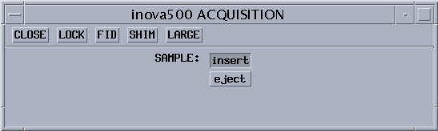
Insert and Lock on a Sample:
- To insert your sample:
- In the VNMR window type e to eject
the reference sample. Remove the reference sample and spinner by gently
grabbing at the spinner and lifting straight up. Remove the reference
from the
spinner.
-
Insert your NMR tube in the spinner
and place in the NMR gauge so that the tube touches the bottom of
the gauge. While holding
the spinner, raise the NMR tube until the solution is centered
about the two white lines (named NMR coil limit in picture below).
For proper sample preparation, see the Preparation
of Samples section.
- Remove the spinner and sample from the gauge by grabbing
the fat part of the spinner and gently place in the upper barrel of
the magnet. IMPORTANT: MAKE SURE THAT EJECTION HAS BEEN ACTIVATED,
YOU WILL HEAR THE GAS PURGING (I.E. A HISSING SOUND)! IF NO
GAS IS HEARD, TYPE e AGAIN. IF IT IS STILL NOT WORKING, CONTACT
THE NMR STAFF AT 3537 or 3478.
- Type i to insert your sample. You
are now ready to Lock on your sample!
- To Lock on your sample:
- Load the default shim set,
which is updated regularly, or retrieve your
own shim values. Wait for the instrument to beep prior to moving
to next step.
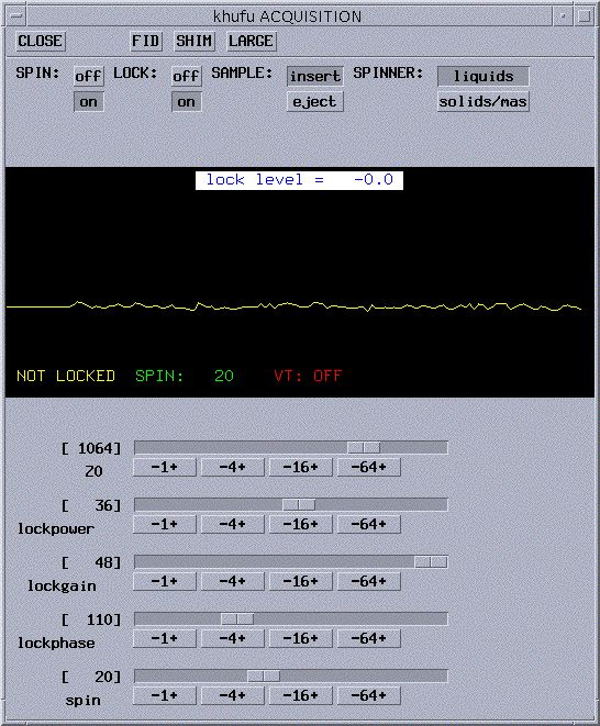
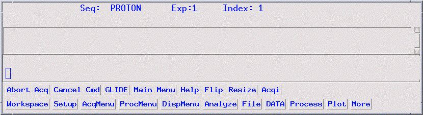
- On the Main Menu screen, click on Acqi (see picture
below). If Acqi is not on the menu screen, type acqi.
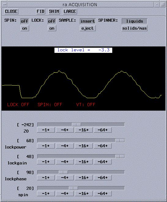
- You will now see a small pop-up window titled ACQUISITION
(see picture below for example).
- Click on Lock.
- The Acquisition window will now show the lock signal plus
the lock controls (see picture below). If the
spin is off, turn it on by clicking on to the right
of SPIN. Adjust the spin rate to 20 Hz. If it doesn't spin, see What
do I do if...
my
sample
is not spinning.
A
note about using the Acquisition window:
ADJUSTING
LOCK AND SHIM VALUES: You can adjust any of the levels in two ways: |
| 1. Using the right mouse button,
click and slowly drag the slide button in the darker gray box next
the bracketed numbers.
Dragging to the left will decrease the number, dragging to the right
will increase it.
|
2. Place the pointer on the button
containing '-number+'
next the value you wish to change. Clicking the left mouse button
will decrease
the value by the value named in the button. Clicking the right
mouse button will increase the value. For example, next to Z0,
I place
the pointer on '-16+' and click the right mouse
button. The value will change from -1488 to -1472. |
- If your sample is already locked, skip ahead to adjust
lockphase. If not, you will probably see a straight yellow line in
the lock window, a lock level below 10, and NOT LOCKED in the corner
(as in the picture above).
- Turn off the lock by clicking the off button
to the right of LOCK:. You should never adjust Z0 when the instrument
is locked.
- Increase lockpower to about 80% of maximum and lockgain
to maximum.
- Using the slide bar for Z0, slowly drag it in one direction
and look for the yellow line to become wavy (i.e. a sine wave as pictured
below) then become a step and stop. If you didn't find it, try the other
direction. You still couldn't find it, see What
do I do if... I can't
lock on my sample.
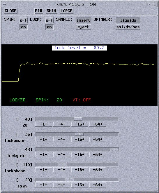
- Now that you have the step , turn the
LOCK on by clicking on to the right of LOCK:. You should
now get a step wave as shown below. Your lock level will be not be steady
because there is too much power being supplied to your sample. You will
need to reduce lockpower until the lock level remains constant.
- Reduce lockpower to the appropriate value. For deuterated
chloroform, 25 is good; for deuterated benzene, acetone, DMF, DMSO, 15
is good. A good lock level is from 40 to 80. If your lock level
is at 100 even though you reduced the lockpower, reduce lockgain. You
will lose lock if you allow the lock level to drop below 15. When this
happens, increase the
lockgain or power and wait a few seconds for the lock to be reacquired.
- Adjust lockphase in units of 4
so that the lock level is as high as you can get it. When adjusting lockphase
and/or shimming, it is best to always adjust until the level drops on
both sides of the maximum. This ensures that you have found the peak
level.
- Your sample is now locked and ready to be shimmed!
Back to Top
Shim and
Save your own Shims for Later Use:
Shimming your sample:
- If you haven't already, in the VNMR window (activate
by clicking in the text box), load shims or retrieve
your own shim values. Be careful about using your own shim values.
If we change the probe, these values will not give good shimming. Also,
due to changes to the spectrometer and its environment over time, old
shim values will be less and less useful. We update the default shims regularly.
- In the acqi window (the window pictured above), click
on SHIM. The window will now looks like:
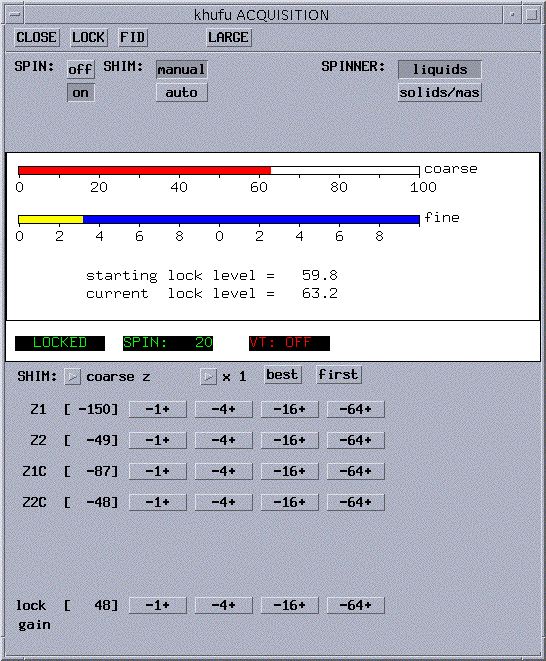
- Start out using manual shimming. To select, click on
manual to the right of SHIM:
- You want to optimize the lock level. This is represented
by the values listed at current lock level and by the horizontal
bars. You will try to get the bars to increase to the right as
much as possible. Don't worry about the color, just try to make
them increase to the right by first adjusting the course Z shims
(Z1C and Z2C) then using the fine controls (Z1 and Z2). A few instruments
don't have Z1C and Z2C. For those instruments, start with Z1 and
Z2 using -64+. A quick procedure is:
- Start with Z1C using -1+ or
Z1 using -64+. Right click on the button repeatedly
and watch the lock level. If
it is increasing,
continue until it is as high as possible. If it is decreasing,
use the left mouse button on -1+ (or -64+
for Z1) to increase the lock level. If you reach a lock level
of 100, reduce the
lock gain (located
at the bottom of the acqi window) until the level is around
30.
- Repeat with Z2C using -1+ or
Z2 using -64+ until lock level is optimized.
- Return to Z1C (or Z1) and reoptimize. Do the
same with Z2C (or Z2) and repeat with Z1C, Z2C until no significant
change
in
the lock level occurs.
- Now repeat the procedure using Z1 and Z2 using
either -4+ or -16+.
- If completed, click CLOSE to
end shimming session and to exit ACQUISITION window.
- If time permits, you can now autoshim.
- Click auto to the right of
SHIM:. From the available choices, select Z1,Z2,Z3.
- Click Start and allow the instrument
to optimize the shims. This will take several minutes. Autoshimming
will be complete when the Stop button changes
to Start. You
can stop at any time by clicking Stop.
- Click CLOSE to end shimming session.
- Your sample is now shimmed and you're ready to acquire
a spectrum!
Saving your own shim values:
- After you have done all the work to optimize your shims,
save them.
- In the VNMR window type svs('filename').
Retrieving your shim values:
Back to Top
Run a Simple 1D Proton or Carbon Experiment: (for a handy Quick
Guide, click
HERE)
- Before beginning to run an experiment, you should be familiar with some
of the basic VNMR commands.
- For a full list of common VNMR commands, click here (PDF
file). The most important for present purposes are:
VNMR
Command
|
Description
|
Typed
Example
|
nt
|
number of transients: Sets the number
of transients (scans) to be acquired. You should always select a multiple
of 4 (e.g. 4, 8, 128). The larger the number of scans, the better the
signal to noise.
|
nt=8
default setting for 1H,CDCl3
|
bs
|
block size: Directs the acquisition
computer, as data are acquired, to periodically store a block of data
on the disk.
|
bs=4
sets the block size to 4 scans. If you are acquiring 100 scans (nt=100),
you can view your spectrum after 4 scans by typing wft.
|
ga
|
submit experiment to acquisition and FT the
result: Performs the experiment described by the current acquisition
parameters and Fourier transforms (wft) the result.
|
|
wft
|
weight and Fourier transform 1D data:
Performs a Fourier transform on one or more 1D FIDs with weighting applied
to the FID.
|
wft
usually used if you stop the acquisition prior to completion or when
loading a saved FID.
|
aph
|
automatic phase of rp and lp: Automatically
calculates the phase parameters lp and rp required to produce an absorption
mode spectrum and applies them to the current spectrum.
|
aph
usually gives well phased spectra
|
f
|
full: Sets the horizontal and vertical
control parameters to produce a display on the entire screen.
|
|
vsadj |
Automatic vertical adjustment: Automatically sets the vertical scale,
vs, in the absolute intensity mode so that the largest peak is at the requested
height. |
vsadj
resets the vertical scale to fit on the screen
|
dscale |
Display scale below spectrum or FID. |
dscale |
aa
|
abort acquisition: immediately aborts
the acquisition.
|
aa
|
sa
|
stop acquisition: stops acquisition
after acquiring current transient.
|
sa
|
su |
submit a setup experiment to acquisition: Sets up the
system hardware to match the current parameters but does not initiate data
acquisition. |
su |
svf('filename')
|
Save FIDs in current experiment: Saves parameters,
text, and FID data in the current experiment to a file.
|
svf('H1_070703')
saves the FID as a file named H1_070703
|
- Acquire a 1D Proton Spectrum:
(Click HERE for 1D Carbon)
- Before beginning make sure you know how to prepare
a sample, reserve NMR time, and log-in
to a spectrometer.
- Lock and shim according to standard procedure.
- Close the acquisition window by clicking Close in the
upper left-hand corner.
- In the VNMR Main Menu screen, click
on Setup =>H1,CDCl3 for
deuterated chloroform. This selects the standard proton parameters.
If you are not using CDCl3, click Nucleus,Solvent => H1,
then choose your solvent. If your solvent is not on the list, click
Other and type in your solvent (e.g. THF).
If you get an error message, just select a solvent that has a chemical
shift similar to your desired solvent. For a list of common NMR solvent
chemical shifts, click here.
- Select the number of scans: The
default setting is 16 (i.e. nt =16). If you need more scans, type nt= #,
where # is the number of scans you desire. Note: nt should
be a multiple of 4 in
order to reduce artifacts (specifically, to reduce quadrature
images). If you are acquiring many scans, you may wish to set the block
size to
4 or
8.
To do this,
type bs=4.
With bs set to 4 scans, the resulting FID will be stored after
ct=4 and you can Fourier transform (wft) or save these
data [svf('filename')].
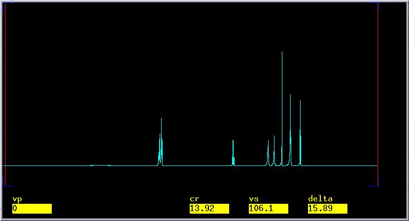
- Start the acquisition: Type ga. The instrument
will automatically check the spinning, adjust the gain, acquire the
spectrum with nt scans, and Fourier transform (wft) the result. When
it's finished, you will hear a beep and see the resulting spectrum,
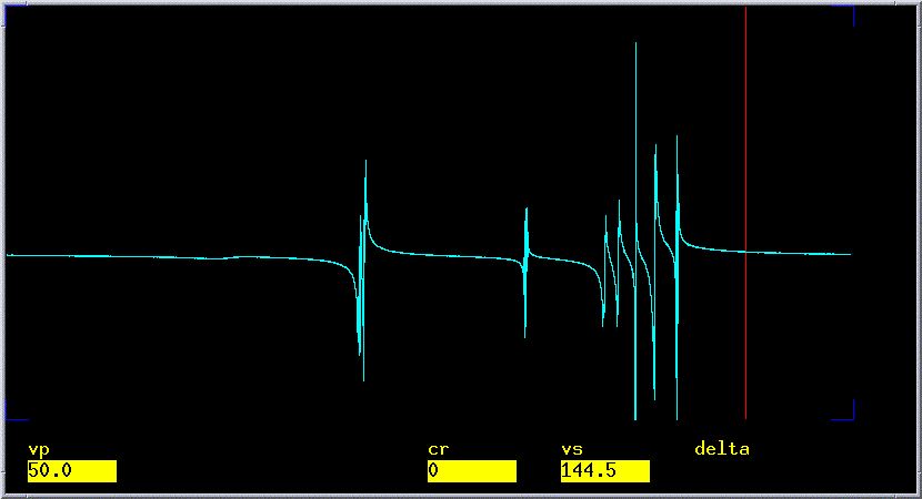
which will generally not be correctly phased. An incorrectly phased
spectrum will have an uneven baseline as in the spectrum below.
- Save the FID: Type svf('filename'), where filename
is your designation for that FID (e.g. svf('dh321_1H'), which contains
my initials, lab book page number, and the nucleus). Now you are ready
to process your data!
- Processing 1D Proton Data: This
may be done at the instrument or at the workstation. We prefer that you use the workstation for processing data so that others
can use the instrument for data acquisition. Log-in and spectral processing
are the same on the datastation as on the instruments. For those users
with one username for all instruments, access to the different spectrometers
is acheived by typing logon in the VNMR command line and following instructions
on screen.
- First you should phase your spectrum.
- To
automatically phase the spectrum: Type aph.
This should give a well phased spectrum with a flat baseline as in
the picture below. In phasing, you are attempting to adjust the spectrum
such that the
baseline on
either side of every peak is even and does not deviate significantly
from the
horizon line.
- If automatic phasing does not fix poor phasing, you
may need to phase it manually.
- Manual Phasing: Click on Phase (second
row middle of Main Menu options buttons. If you don't see it,
click Main Menu => Display => Interactive => Phase).
Type lp=0 to reset the First-Order Phasing to zero.
Increase the scale using the middle mouse button such that the
base of the biggest peaks are clearly visible.
- Adjust Zero-Order Phasing: Using the left
mouse button, click on the middle of the largest peak on
the right side
of
the spectrum
and
drag
the
mouse
either
up
or
down. You will notice the phase changing for the selected
peak. If the baseline is becoming even, continue to drag
the mouse
until it is as even as you can get. If the baseline is
getting worse, drag the mouse in the opposite direction.
If you come
to the edge of the spectrum window and it's still not phased
properly, click Phase again and continue
to drag in the same direction as previous starting from
the opposite edge
of the window (i.e. I dragged the mouse up and came to
the top of the window, so I click Phase and
begin dragging up from the bottom of the window).
- Adjust First-Order Phasing: Using the left
mouse button, click on the middle of the largest peak on
the left side of the spectrum and drag up or down. Proceed
as with Zero-Order phasing; remember, you are trying to get
the baseline even.
Once you get it as good as possible, return to the right
side of the spectrum and rephase the biggest peak again.
Repeat until optimum.
- Reference your Spectrum:
Spectra are generally referenced
to the residual protio signal from the deuterated solvent. Click Solvent
Reference to determine the chemical shift for your solvent
(CDCl3 is a singlet at 7.24 ppm, acetone is a pentet at 2.04
ppm). The standard
parameters that you chose to setup the experiment referenced
the spectrum to a
preset
value.
This
value
will
be close
to the correct chemical shift of your solvent as long as you
specified the correct solvent during setup.
Find your solvent peak: Type dscale. Locate
the region for your solvent peak and expand it. For deuterochloroform,
the region would be around 7.24 ppm. Expand on the desired region;
click the left mouse button at the left-most point of
the desired expansion (you will see a red line) then click the
right mouse button on the right-most point of the expansion (you will
see
two red lines denoting the region to be expanded) and click Expand.
To expand further, click the left mouse button then the right and click Expand.
(To return to the full spectrum, click Full.)
Reference your solvent: With the left mouse button
click at the top of your solvent peak. Type nl. This
brings the cursor to the top of the nearest peak. Type rl(solvent
chemical shiftp) (e.g. rl(7.24p) for CDCl3
or rl(7.15p) for
benzene-d6 or rl(2.04p) for acetone-d6). Remember for
multiplets like acetone-d6, reference the middle peak.
Integrate your Spectrum:
Given ample time for the induced magnetization to relax
(5*T1), peak areas are directly proportional to the number of protons
responsible for the given peak(s), thus making it possible to determine
the relative number of protons in a given system. Deviation from
a direct relationship can be due to insufficient time for complete
relaxation.
Usually sp2 hybridized centers will have longer T1s then sp3 centers
and thus you may get integrated values for sp2 centers that are less
then they appropriate. To reduce this phenomenon, increase d1 (e.g. d1=30). A
flat baseline and consistent, level integrals are very important.
Integration
Quick Reference
|
If you want to...
|
then you should do this...
|
Clear integral resets
|
Type cz |
Increase spectrum size when in integration
mode
|
Type vsadj for vertical scale adjustment to maximize
the largest peak in the region.
If you need to increase further, click Full Integral => No
Integral and adjust the peak height using middle mouse
button. Turn integral on by clicking Part Integral.
|
Increase integral size
|
Whenever the integrals are displayed, the middle mouse button controls
the size of the integrals. Clicking on the screen above the integral
will increase the integral to that position. Clicking below the spectrum
will decrease all integrals by a half. |
Change integral position
|
Type io=30 or appropriate value. |
View integral values
|
Type vp=12 dpir |
Perform a baseline correction
|
Type bc |
- View and Level your integral: click Part
Integral in the Interactive Menu (If you don't see this
button, click Main Menu => Display => Interactive => Part
Integral). You will now see a stepped green line across
the entire screen. Type f cdc dc and hit Return. If
your integral trace does not have a flat baseline, you will have
to adjust it manually. Click on Lvl/tlt.
With the left mouse button click on the left-most integral (step)
and
drag up to increase the slope or down to decrease it. You want
the slope
of the integral to be zero at the left edge of the integral trace.
Click on the right-most integral step and drag it in the appropriate
direction such that the overall slope of the integral is as near
zero as possible (i.e. a flat line between peaks). When done
click on Box.
- Reset integral for individual peaks: Type f.
Expand around a desired region for integrals. Click on Resets.
Starting from the left-hand side and using the left mouse button,
click on the baseline around each desired peak set (e.g. a triplet,
quartet). Integrated areas will have a solid green line and unintegrated
areas have a dashed line. Once completed with a section, click Full,
expand around the next region of interest and click Expand => Resets.
Repeat process of setting your individual integrals. If you want
to change a single reset point, place the cursor over that point
and click the right mouse button. If you make a mistake and need
to start over, type cz to
clear the integral reset points. When you are done, you can type bc;
this is a baseline correction based on the integral regions that
are
nulled in your spectrum, but be careful because a simple bc can
cause significant dips around the peaks. To undo the bc, just
type wft.
- Reference your integral: Look
for a peak that you think you know the number of protons (e.g. a
singlet around 2 ppm could be an acetate group and therefore should
be 3 protons). Expand around the peak and set the cursor anywhere
under its integral by clicking with the left mouse button. Click Set
int and type in the new integral value (e.g. for the acetate
group, I would type 3).
- View your integral values: Type vp=12.
This moves the spectrum and scale up by 12mm. Type dpir. This displays
the integral values. If the values are overlapped, you will need
to expand the region and retype dpir. Your spectrum is now
integrated and you're ready to peak pick!
Peak Picking: Note: Any time
you want to replot the peak values, type ds first to redraw
the spectrum without the old peak values.
Peak Picking
Quick Reference
|
If you want to...
|
then you should do this...
|
display all peaks
|
Type dpf |
display only positive peaks
|
Type dpf('pos')
|
increase sensitivity on peak picking
|
Type dpf(0). The default is 3; any value greater then
that will decrease sensitivity. |
clear peak labels
|
Type ds. |
set peak threshold
|
click on Th and use left mouse button to drag
the threshold line (yellow) to the desired height. |
display a peak list
|
Type dll. The peak list will apply in the gray window
below the spectrum window. If you can't see the gray window, click Flip. |
Peak picking is important because it allows you to
print the peak locations and calculate coupling constants. The yellow
line designates the threshold below which no peaks are picked.
Set your peak threshold: With
the full spectrum displayed, click Th. You will
see a yellow line across the screen. Using the left mouse button,
click and drag the yellow line to the level just below the smallest
peak you wish to have displayed.
Display peak labels: Type dpf or
variant (see Table above). If you need greater peak sensitivity,
type ds dpf(0). You are now ready to print your spectrum!
- Printing Simple Proton Spectra:
Printing
Quick Reference
|
String together any of the commands
listed below in any order followed by page to print
what you want. Whatever is displayed on the screen will be
printed.
For example, I typically use: pl
pscale pll pltext(150,150) pir page.
|
Command
|
Action
|
pl
|
print spectrum
|
pscale
|
print scale
|
pll
|
print line list, which includes frequency in
Hertz for calculating J-values
|
ppf
|
print peak frequencies
|
pir
|
print integral values (vp must be greater than
10: type vp=12)
|
pltext
|
print text. To plot in the upper right corner,
type pltext(150,150), this is necessary when you are printing
a peak list (i.e. pll).
|
pap
|
print all parameters
|
- Add Text to your Spectrum: Type text('text
here\\more text more'). The \\ opens a new line of text, which
is similar to hitting Enter in Word. Your text will appear in the
gray window below the spectrum (click Flip to
view window). For example, I might type text('dh300\\V-500
CDCl3 1H NMR\\07-10-08'), which would look like (if printing
using pltext(150,150)):
dh300
V-500 CDCl3 1H NMR
07-10-08
- Print your Spectrum: Display
the region you desire to print. To print an exact region, type sp=#p
wp=#p, where the sp=#p is the value in ppm where it will begin
the display and wp=# is the width in ppm of the desired region. For
example, I want to print the region from 6.2 ppm to 8.2 ppm, so I
type sp=6.2p wp=2.0p.
- Type vsadj if you want the tallest
peak to be scaled to fit the screen.
- To print, see the Quick reference above for
various commands; type, for example, pl pscale pltext ppf
page. This will print the spectrum, scale, text, and peak
frequencies.
- NOTE: page must be typed at the end
of each printing request in order to print the spectrum!
- When completed, be sure to exit VNMR and log-out properly.
Click here to view log-off procedure.
- To print stacked spectra: You
will need to create an arrayed dataset, which will allow you
to view and print all stacked spectra.
- Load the spectra in exp1 and add them to an
array:
- type jexp1 - join experiment
1
- type clradd - clear the add/sub
buffer in exp5. This will erase anything in exp5.
- click Main Menu => File and
select the first desired spectrum and click Load.
- type add - adds FID to add/sub
buffer.
- For adding all additional spectra, click File,
select the desired spectrum, click Load,
and type add('new').
- Join exp5 and create array parameters:
- type jexp5 - join experiment
5.
- type gain='y' - turns off autogain,
which is not allowed in arrayed experiments.
- type d2=1,2,3... - sets arrayed
variable. Use same number of variables as spectra.
- type calcdim - calculates the
array dimension.
- type groupcopy('current','processed','acquisition') -
updates parameters.
- type ai - resets to absolute
intensity mode.
- type wft dssa - Fourier Transform
all FIDs and display stacked spectra.
- type svf('your filename') to
save the arrayed spectra.
- You may need to adjust the phasing.
If phasing is incorrect, type ds(1) (this
displays the first spectrum), or click Interactive.
Type aph.
- To adjust the scale of each spectrum:
type ds(spectrum number) (where spectrum number
is an integer. For the first spectrum, spectrum number
is 1: ds(1); for the second spectrum, spectrum
number is 2: ds(2); etc.). Adjust the scale
as usual. To check, type dssa.
- To print, use standard printing commands
except replace pl with pl('all').
- To Print an Expanded Region or
inset with your Spectrum:
- Process your spectrum as you normally would
(see Processing 1D Proton Data) and type pl pscale
pir etc. but do not type page.
The page command sends the job to the printer.
You want to hold this job until you add your inset(s).
- Put the cursors around the region for which
you wish to print an expansion.
- Type inset. The expanded view
will appear on the screen. This view is now interactive
and can be manipulated like usual. The full spectrum is
no longer interactive.
- Use the left mouse button to set
the horizontal position.
- Use the middle mouse button to set
height.
- Use the right mouse button to set
size.
- Use the vp command to set vertical
position (e.g. type vp=40 to set the inset
at 40 mm)
- If you expand the inset and wish
to reposition the new expansion, click sc
wc and move as described before.
- To print the inset: type pl pscale pir etc.
If you would like another inset, repeat the process described
above ensuring that you type pl pscale pir after
each inset. When completed, type page.
Back to Top
Acquire a 1D Carbon Spectrum:
- Before beginning make sure you know how to prepare
a sample, reserve NMR time, and log-in
to a spectrometer.
- Lock and shim according
to standard procedure.
- In the VNMR Main Menu screen, click on Setup =>C13,CDCl3 for
deuterated chloroform. This selects the standard proton parameters.
If you are not using CDCl3, click Nucleus,Solvent => C13,
then choose your solvent. If your solvent is not on the list,
click Other and type in your solvent (e.g. THF).
If you get an error message, just select a solvent that has a
chemical shift similar to your desired solvent. For a list of
common NMR solvent chemical shifts, click here.
- Once you have selected the solvent, type su.
- Select the number of scans: The
natural abundance of
13C is 1.108%, which means that roughly
1 in every 100 carbons will be NMR active. You will need more
sample and scans than
1H spectra. Type nt= 256.
Note: nt should be a multiple of 4 in order
to minimize noise. Since
you are acquiring many scans, you may wish
to set the block size to 4 or 8. To do
this, type bs=4 or bs=8. With
bs set to 4 scans, the resulting FID will be stored after ct=4
and you can Fourier transform (wft) or save these data
[svf('filename')] at any time. This is good to check
the evolution of signal to see if you have enough time to get
good s/n.
- Set your relaxation delay: Carbon
T1s can be quite long, especially for carbonyls and quaternary
carbons (these can be anywhere from a few seconds to hundreds
of seconds!). Pulsing too frequently (i.e. too short relaxation
delay) will saturate signals from carbons with long T1s, so
it is therefore advisable to increase the relaxation delay
for aromatic, alkenyl, or carbonyl containing compounds. This
is set with d1. Setting d1 to 1 to 10 seconds should be sufficient.
To do this, type d1=1 or a different value.
- Start the acquisition: Type ga.
The instrument will automatically check the spinning, adjust
the gain, acquire the spectrum with nt scans, and Fourier transform
(wft) the result. When it's finished, you will hear a beep and
see the resulting spectrum, which will generally not be correctly
phased.
- Phasing and Referencing is similar
to the procedure with Proton: Click Here for
Phasing and Referencing. Make sure that
you reference to the carbon chemical shift
(e.g. Chloroform-d appears
as a triplet centered at 77.0 ppm).
- When completed, be sure to exit VNMR and log-out
properly. Click here to view log-off procedure.
Back to Top
Determine number of protons attached
to each carbon (DEPT):
Distortionless Enhancement
by Polarization Transfer
(DEPT) is an experiment that utilizes a polarization transfer from one
nucleus to another, usually proton to carbon or other X nucleus, to increase
the signal strength of the X nucleus. Furthermore, by varying the length
of the last proton pulse from 45 to 135 degrees, the multiplicity of the
carbon or X nucleus can be determined (i.e. depending on the pulse the
signal for a methine, methylene, or methyl will either be a positive, negative,
or null signal. See table below). Addition and subtraction of the various
DEPT spectra will give the multiplicity of each carbon. Remember, since
quaternary carbons have no attached protons, they will show no signal.
Relative Intensities
from DEPT
|
Spectrum #
|
Pulse Angle
|
C (quaternary)
|
CH (methine)
|
CH2 (methylene)
|
CH3 (methyl)
|
1
|
45
|
0
|
0.707
|
1
|
1.06
|
2,3
|
90
|
0
|
1
|
0
|
0
|
4
|
135
|
0
|
0.707
|
-1
|
1.06
|
- Run a DEPT Experiment:
This is an arrayed experiment which will run 4 separate
DEPT experiments: DEPT 45, 2 DEPT 90s with slightly different pulse
widths, and a DEPT 135.
- Acquire a quick 13C spectrum (Click
Here for Procedure) and reference your solvent. Solvent peak is nulled
in DEPT.
- Type DEPT.
- Type nt=64 or larger number if necessary.
- Type go. A total of 4 FIDs, each having
64 scans, will be acquired.
- After acquisition is complete, save your file
[i.e. type svf('filename')]
- Process and Print DEPT Data:
- Type wft: performs a weighted Fourier transform
of all 4 FIDs.
- Type ds(1) to display the first spectrum
(this is the DEPT 45 spectrum; all peaks are positive) and phase
it (for help with phasing, click here).
- Type dssa to view all 4 spectra stacked
vertically. You may want to scale the spectra to fit. To do this,
type ds(#), where # is the number of the spectrum you wish
to scale. Scale the selected spectrum as usual using the middle mouse
button. Return to the stacked plot with dssa.
- Type ds(1), click th and
position the yellow threshold line below all the peak tops.
- Type fp: this stores the peak frequencies
in memory.
- Type dll: displays the line list.
- Type DEPTP: this is a macro that automatically
processes and prints the DEPT data.
- Printing individual DEPT Spectra:
Sometimes I have found it beneficial to print the individual
DEPT spectra. With the help of the DEPT table above, it is rather straightforward
to determine the carbon multiplicity. See the DEPT table above to see
which spectrum gives which DEPT experiment. For example, from the second
and third spectra (to view type ds(2) or ds(3)), which
are DEPT 90 spectra, I will get only the methine carbons and from the
fourth spectrum, I get the methylene carbons because they are the negative
peaks.
- Type ds(#), where # is the number of the spectrum
you wish to print. Manipulate and plot as you would a standard Carbon
spectrum. To plot, type, for example, pl pscale ppf pltext page.
- When completed, be sure to exit VNMR and log-out
properly. Click here to view log-off procedure.
Back to Top
Determine 1H-1H connectivity (COSY): (PDF Version available here!)
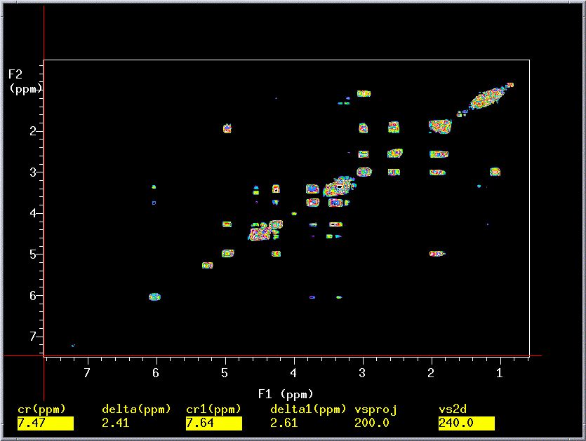
COrrelation Spectroscopy (COSY)
is a 2D NMR technique which gives correlations between J-coupled
signals by incrementing the delay between two 90 degree proton pulses.
The resulting 2D spectrum is generally displayed as a contour plot (see
below), which is similar to a topographical map. When looking at a contour
map, you are actually looking down at a cross-section (slice) of a 3D-image
of an NMR spectrum. The usual 1D spectrum is traced on the diagonal of
the plot and any peaks that are not on the diagonal represent cross-peaks
or rather correlation peaks that are a result of J-coupling. Thus,
by simply tracing a rectangle using the diagonal and cross-peaks as vertices
you will know which protons are coupled to each other. Standard COSY experiments
require phase cycling to remove unwanted signals and thus can be quite
time consuming. This can be circumvented using gradient selected COSY (gCOSY),
which utilizes pulsed field gradients to destroy unwanted z-magnetization
and hence their associated signals (axial peaks). Quality gCOSY spectra
can be acquired in as little as 20 minutes! All our instruments except
the Geminis are equipped to do gradient selected spectroscopy.
- Running a gCOSY Experiment:
- Join experiment 1 by typing jexp1.
- Type vttype=2 su to enable temperature control.
- Type temp and slide the bar in the pop-up
window to 25. This sets the temperature to 25
degrees Celsius. It is important to maintain
a
constant temperature
while acquiring a gCOSY.
- Shim well, acquire and process a 1D Proton spectrum
(click Here for instructions).
- Note the left-most and right-most peaks from
your spectrum (for example, 8 and 2 ppm).
- Type svf('filename') to save the spectrum.
- Type jexp2: this joins experiment 2. If
you get an error message, click Workspace => Create
New.
- Type mf(1,2). This moves the FID from exp1 to exp2.
- Turn off the spin and adjust the lock level to 50%
or higher using lock gain and lock power. Be sure not to saturate
your lock signal with too high lock power. The lock power is too
high if it has large fluctuations.
- Type gCOSY: This loads the acquisition parameters.
- Type setwindows: This is an in-house macro
that allows you to easily set the sweep width in both dimensions.
You will need to enter the following information:
- "Enter the 1H left ppm limit:" Use
a value 1 ppm greater than your left-most 1H peak. If your
peak is 8 ppm, then type 9.
- "Enter the 1H right ppm limit:" Use
a value 1 ppm less than your right-most 1H peak. If your peak
is 2 ppm, then type 1.
- Type nt=#, where # is the number of scans
you wish.
- Type time and note the value. You can increase
nt and check time again to fill your allotted instrument time.
- Type go (please do not type ga).
- Data Manipulation:
- Type setLP1 sinebell wft2d: This performs
the 2-dimensional Fourier transform and the color map will be displayed.
The color
map is your 2-D spectrum with the levels displayed using different
colors. Use the following table as a guide to color map navigation.
Type d2d to display a contour map that matches the printout.
Interacting
with the 2-D Color Map/Contour Map
|
To do
the following...
|
You should...
|
Increase/Decrease the scale
|
Click on either vs+20% or vs-20% or
type vs2d=vs2d*1.5 and click Redraw.
The typed command increases the display by a factor of 1.5. You
can use a larger number if you like (e.g. vs2d=vs2d*2,
increases by a factor of 2.
|
Change the number of color levels
|
Use the middle mouse button to click on the
color scale to the right of the color plot. Click on the smaller
number to increase the number of colors displayed.
|
To expand on a region
|
Ensure that you are in the interactive mode;
if not, click Main Menu=>Display=>Color
Map. Click with the left mouse button on the left-most
point of your desired region. Click with the right mouse button
on the right-most point. Click on Expand.
|
To expand an exact region
|
Type sp=#p wp=#p (for the F2 dimension,
usually vertical) and sp1=#p wp1=#p (for the F1 dimension,
usually horizontal), where # are the numbers in ppm for the region
of interest. sp designates the start of plot and wp is the width
of the plot. You will need to click on Redraw to
update the screen. For example, I want to expand the region between
1 and 4 ppm in F1 and between 2 and 4 ppm in F2, I would type sp=2p
wp=2p sp1=1p wp1=3p, then I click Redraw to
see the result.
|
To reference the 2-D spectrum
|
Expand the region of interest. Click Hproj(max) for
the horizontal projection and Vproj(max) for the
vertical projection. Place the cross-hair cursor on the diagonal
position you wish to reference (the projections will help you to
orient the cross-hair). Type rl(#p) rl1(#p), where # is
the value in ppm you want to be the reference. rl sets the F2 dimension
reference and rl1 sets the F1 dimension reference. |
Redisplay the spectrum
|
Click on Redraw.
|
Display a projection of the 1D spectrum on
the side of the 2-D plot
|
Click Proj, then click Hproj(max) for
the horizontal projection or Vproj(max) for
the vertical projection. Use the middle mouse to adjust the scale.
|
Display a trace of the 2-D plot
|
Click Trace and use the left mouse button to
drag the cursor. |
View the contour plot
|
Click Main Menu=>Display=>Contour
|
Increase number of levels on contour plot:
Interactive plot
|
Type, for example, dconi('dpcon',15,1.2).
The dpcon flag is for displaying the contours. The first number
(15, in this case) is the number of contour lines (default is
4). The second number (1.2, in this case) is the relative spacing
intensity (default is 2). You can input different numbers if
you wish, but the second number must be greater than 1.
|
Increase number of levels on contour plot:
Non-interactive plot
|
Type, for example, dpcon(15,1.2).
The dpcon flag is for displaying the contours. The first number
(15, in this case) is the number of contour lines (default is
4). The second number (1.2, in this case) is the relative spacing
intensity (default is 2). You can input different numbers if
you wish, but the second number must be greater than 1.
|
- Autoprinting your gCOSY with Projections
generated from COSY:
- Display the region of interest and click Autoplot:
This plots your COSY with the projections generated from the
1-D data subsets. The indirectly detected dimension will have
low resolution and thus, the projection for that dimension
(usually F1) will have broad peaks. For better resolution projections,
use the following procedure.
- Printing your gCOSY with 1-D Spectrum
as Projections:
Open your COSY Spectrum. Click Main Menu=>Display=>Size=>Center.
- Join another experiment and retrieve the 1-D
spectrum:
- Type jexp1 or any other experiment
number.
- Load the 1-D spectrum; Fourier transform
(wft), and phase (aph).
- Type jexp2 or join the experiment number
where your COSY resides:
- Click Display=>Contour and
expand, scale, etc. the region of interest (refer to table
for interacting with the color or contour map).
- Type plgcosy and follow the directions
on the screen: This is our in-house macro that prints your
desired 2-D spectrum with high-resolution 1D plots on the
sides.
Back to Top
- LOGGING OFF OF INSTRUMENT SESSION:
- After you are done, you must leave the instrument as
you found it.
I. In the VNMR window, type e. Eject your sample, remove it from the spinner,
put back the reference sample in the spinner, and use the depth gauge to
set the proper height.
II. Place spinner with reference sample in magnet bore
III. Type i. Insert the reference sample.
IV. In the VNMR window type exit.
V. After VNMR closes, right click on the background, and choose log
out… at
the bottom of the menu.
VI. Click OK to completely exit the session.
Run a Homonuclear
Decoupling (HOMODEC) Experiment: (PDF available here)
This is a simple and quick means of determining
if two resonances are coupled. The HOMODEC experiment is most effective
for relatively simple spectra where the couplings are, at least, somewhat
resolved. The experiment consists of irradiating a selected resonance with
a low power decoupler, which will eliminate any couplings to that resonance.
By comparing the resulting spectrum to that without decoupling, it is easily
determined which resonance(s) are coupled to the irradiated peak.
- Acquire a 1H NMR spectrum. For a procedure, click HERE.
- Type HOMODEC. This enables homodecoupling.
- Type ds to display the spectrum and expand around the desired
resonance you wish to irradiate (i.e. the one that you want to determine
coupling).
- Click on Cursor and place the cursor on
a position in the spectrum that contains no peaks within 0.3 ppm. This
is a reference spectrum.
- Type sd. This resets the decoupler offset to the cursor
location.
- Expand and place cursor on your desired peak to be decoupled
and type sda.
Repeat using sda for all peaks you wish to decouple.
- Choose your number of scans and type ga.
- Type wft ds(1) vsadj and, if necessary, manually
phase. Ignore the irradiated peak because it will not phase correctly.
- If the irradiated peak is still positive and contains splitting,
you may want to increase the decoupler power. Type dpwr=30 and repeat the
experiment. Do not increase dpwr above 40.
- Type vs=vs/#, where # is the number of spectra in the
array.
For example, if you did one reference and 2 decoupled spectra, type vs=vs/3.
- Type f full
dssa. This displays the spectra in a vertical stack.
- Expansion is the same as with 1D spectra, but you must type
ds first.
- To plot all stacked spectra, type pl('all') pscale pltext
page.
- To plot selected spectra, type pl(1, #) pscale pltext
page, where # is the number of the spectrum. For example, if I wanted to print
the reference and the third spectrum, I would type pl(1,3) pscale pltext
page.
*Portions of this page were adapted from procedures
by Long Lee and Kermit Johnson.